Linear Attention Basics

In the previous “boring” post, we discussed the traditional softmax attention mechanism and its limitations, particularly in terms of $O(n^2)$ computation cost during inference. We also reviewed the “age-old” RNNs, which have $O(n)$ computation cost but struggle to be trained in parallel.

Now, let’s see something interesting:

• Attention without softmax = RNN
• RNN with rank-1 hidden matrix and no reflection = Attention

This is wild!!!

Dereivation

attention -> RNN

Let’s start with the softmax attention mechanism:

(for simplicity, we omit the scalar $d_k$ in the attention formula)

Without softmax, we have:

Let

and

, we have:

Which is a linear RNN!

RNN -> attention

Now, let’s start with a simple RNN:

where $f(\mathbf{x}_t) = (\mathbf{x}_t \mathbf{W}_k)^T (\mathbf{x}_t \mathbf{W}_v) = \mathbf{k}_t^T \mathbf{v}_t \in \mathbb{R}^{d \times d}$ , $\mathbf{W}_h = \mathbf{I}$, and $f_O(\mathbf{h}_t) = \mathbf{q}_t \mathbf{h}_t = \mathbf{x}_t \mathbf{W}_q \mathbf{h}_t$.

Now, the hidden state is no longer a vector, but a $d \times d$ rank-1 matrix. Together with another hidden state $\mathbf{k}_t$, we can rewrite the RNN as:

Unfolding the RNN, we have:

This is the attention output (linear combination of value vectors)!

So what?

What an exciting result! It allows us to train our models in “attention” mode, and then switch to “RNN” mode for inference. But wait, there’s more! Take a look at the “attention” formula:

The terms

and

are independent of $t$. Therefore we can pre-compute these terms and store them in a cache (in a sense of dynamic programming), allowing us to compute the attention output in $O(1)$ time at each time step. In this way, the total computation cost for processing a sequence of length $n$ is $O(n)$, which is much more efficient than the traditional softmax attention mechanism.

Another view of this is that when we drop the softmax, instead of computing $(\mathbf{Q}\mathbf{K}^T)\mathbf{V}$, which takes $O(n^2d)$ multiplications, we compute $\mathbf{Q}(\mathbf{K}^T\mathbf{V})$, which takes $O(nd^2)$ multiplications.

Spoiler: what if we have a causal mask? It’s sad that we can no longer use the associativity of matrix multiplication with a causal mask. Therefore it’s hard to parallelize the computation in time dimension. See the next post for more details and a solution.

Attention Free Transformer

Before we see the RWKV architecture, it’s worth paying a glance at the attention-free transformer (AFT), since it provides insight into the RWKV architecture.

AFT-Simple

Firstly, let’s see the AFT-simple architecture:

where $\sigma_q(\mathbf{q}_t)$ is a non-linear function(sigmoid as default) of the query vector $\mathbf{q}_t$, $\odot$ denotes element-wise multiplication, and the division is also element-wise.

With the knowledge of linear attention, now we can see that the values of

and

are independent of $t$, thus can be cached to save computation cost. Furthermore, all operations are element-wise, the hidden state reduces to a vector, and the computation cost is $O(n)$.

The RNN form of AFT-Simple is:

AFT-Full

AFT-Full introduces a learable “pair-wise position bias” to AFT-Simple:

where $w_{t,j} \in \mathbb{R}$ is the learnable position bias for the $j$-th token at time step $t$. Together they form a $N \times N$ matrix. The interpretation of this is that

. Therefore $w_{t,j}$ acts like an input gate for the $j$-th token at $t$.

Note that the AFT-Full architecture cannot be unfolded into a RNN, since the position bias $w_{t,j}$ is not independent of $t$. And the computation cost is still $O(n^2)$.

RWKV v4

Finally, we are ready to see the RWKV v4 architecture. The RWKV v4 architecture looks similar to AFT-Full, but with a few key differences:

1. The position bias $w_{t,j}$ is replaced with a learnable “pair-wise position bias” $\mathbf{w}_{t,j} \in \mathbb{R}^{d}$, which is a vector instead of a scalar (each element is responsible for the entire sequence in a channel).

2. To “circumvent any potential degradation of $\mathbf{W}$”, the RWKV v4 architecture uses another vector $\mathbf{u}$ to attend to the “current” tokens (while the “past” tokens are governed by $\mathbf{W}$). This design will be seen clearly in the WKV operation.

The WKV operation

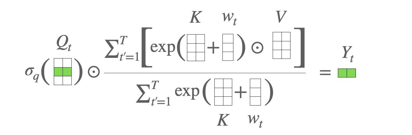
For coherence, I skipped some important innovations in the RWKV v4 architecture, such as the “token-shift” operation; we will see them after the illustration of the WKV operation. Now it’s time to see the (causal) WKV operation, which is defined as:

From the expression of the first term of the numerator, we can see that the $e^{k_j}$ is now affected by a decayed term $e^{-(t-1-j)w}$, which diminishes the influence of the “past” tokens as $j$ increases.

This is a key difference from the AFT-Full architecture, where the position bias $w_{t,j}$ is independent of $j$. The second term of the numerator is the “current” token, which is governed by $\mathbf{u}$ and $\mathbf{W}$. The denominator is the sum of the two terms, which normalizes the output. The WKV operation can be interpreted as a linear attention mechanism, where the “past” tokens are attended to with a decayed weight, and the “current” token is attended to with a learnable weight. This allows the model to learn more complex relationships between the tokens in the sequence.

Question: What’s the role of the decay term?

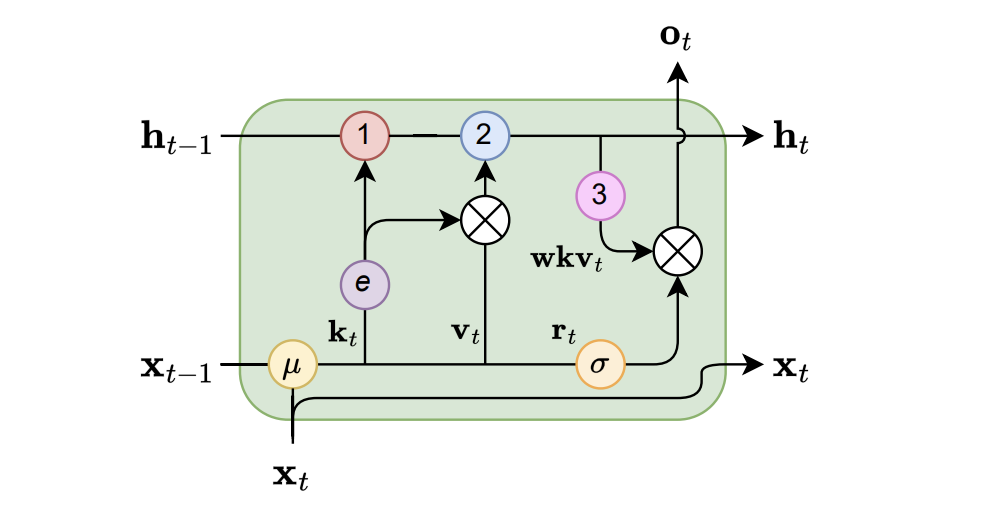
Written in RNN form, the WKV operation is:

Now it’s easier to see the role of the decay term: it allows the model to learn a “forgetting” mechanism, which is similar to the forget gate in LSTMs. The decay term $e^{-w}$ diminishes the influence of the “past” tokens as $t$ increases, allowing the model to focus more on the “current” token.

However, $e^{k_t}$ can be large, and the above equation may cause overflow. To avoid this, we use a trick to constrain the values of the two “coefficients” to be in (0, 1]:

The same trick is applied to update $a_t$ and $b_t$:

Since channels are independent, the above equation can be computed in parallel for each channel. To see it clearly, let’s dive into the official implementation of the WKV operation:

 1
 2
 3
 4
 5
 6
 7
 8
 9
10
11
12
13
14
15
16
17
18
19
20
21
22
23
24
25
26
27
28
29
30
31
32
33
34
35
36
37
38
39
40

// RWKV v4 WKV operation (forward)
    /*
    dim3 threadsPerBlock( min(C, 32) ); 
    dim3 numBlocks(B * C / threadsPerBlock.x);
    kernel_forward<<<numBlocks, threadsPerBlock>>>(...);
    */
template <typename F>
__global__ void kernel_forward(const int B, const int T, const int C,
                             const F *__restrict__ const _w, const F *__restrict__ const _u, const F *__restrict__ const _k, const F *__restrict__ const _v,
                               F *__restrict__ const _y) {
    const int idx = blockIdx.x * blockDim.x + threadIdx.x;
    const int _b = idx / C;
    const int _c = idx % C;
    const int _offset = _b * T * C + _c;

    F u = _u[_c]; // channel-wise
    F w = _w[_c]; // channel-wise
    const F *__restrict__ const k = _k + _offset;
    const F *__restrict__ const v = _v + _offset;
    F *__restrict__ const y = _y + _offset;

    F p = 0, q = 0, o = MIN_VALUE;
    // p and q are running sums divided by exp(o) (to avoid overflows)
    for (int i = 0; i < T; i++) {
        // O(n) complexity
        const int ii = i * C;

        F no = max(o, u + k[ii]);
        F A = exp(o - no);
        F B = exp(u + k[ii] - no);
        y[ii] = (A * p + B * v[ii]) / (A * q + B);

        no = max(w + o, k[ii]);
        A = exp(w + o - no);
        B = exp(k[ii] - no);
        p = A * p + B * v[ii];
        q = A * q + B;
        o = no;
    }
}

After the WKV operation, an output gate $\sigma(r_t)$ is applied to the output of the WKV operation, where $\sigma$ stands for the sigmoid function, and $r_t$ is generated from the input token $\mathbf{x}$:

This explains the name “RWKV”.

Token-shift

Another innovation in the RWKV v4 architecture is the “token-shift” operation, which acts like a “short convolution” interpolating two adjacent tokens. The token-shift operation is defined as:

Or in a unified form:

Token shift tell the model how to treat new tokens by interpolating between the current and previous token representations. In essence, it can be viewed as a convolution with kernel size 2 (The FFN block in the transformer architecture can be viewed as a convolution with kernel size 1), which enhances the model’s ability to capture local patterns in the sequence.

Note: Mamba also proposed a similar idea, i.e., “causal conv1d”, applied to the input embedding before the SSM block.

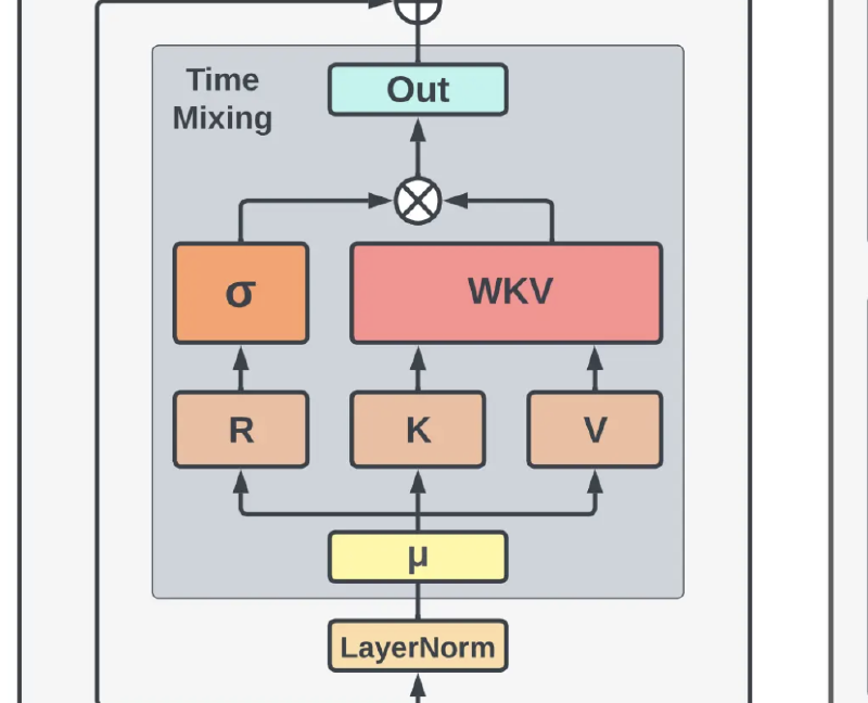
Overall architecture

The overall architecture of RWKV v4 is shown below:

In which the “Time Mix” block is the rwkv operation, and the “Channel Mix” block is similar to the FFN block in the transformer architecture, yet equipped with token-shift as well.

where $\max(k’_t, 0)^2$ is the square of the ReLU activation of $k’_t$.

Summary

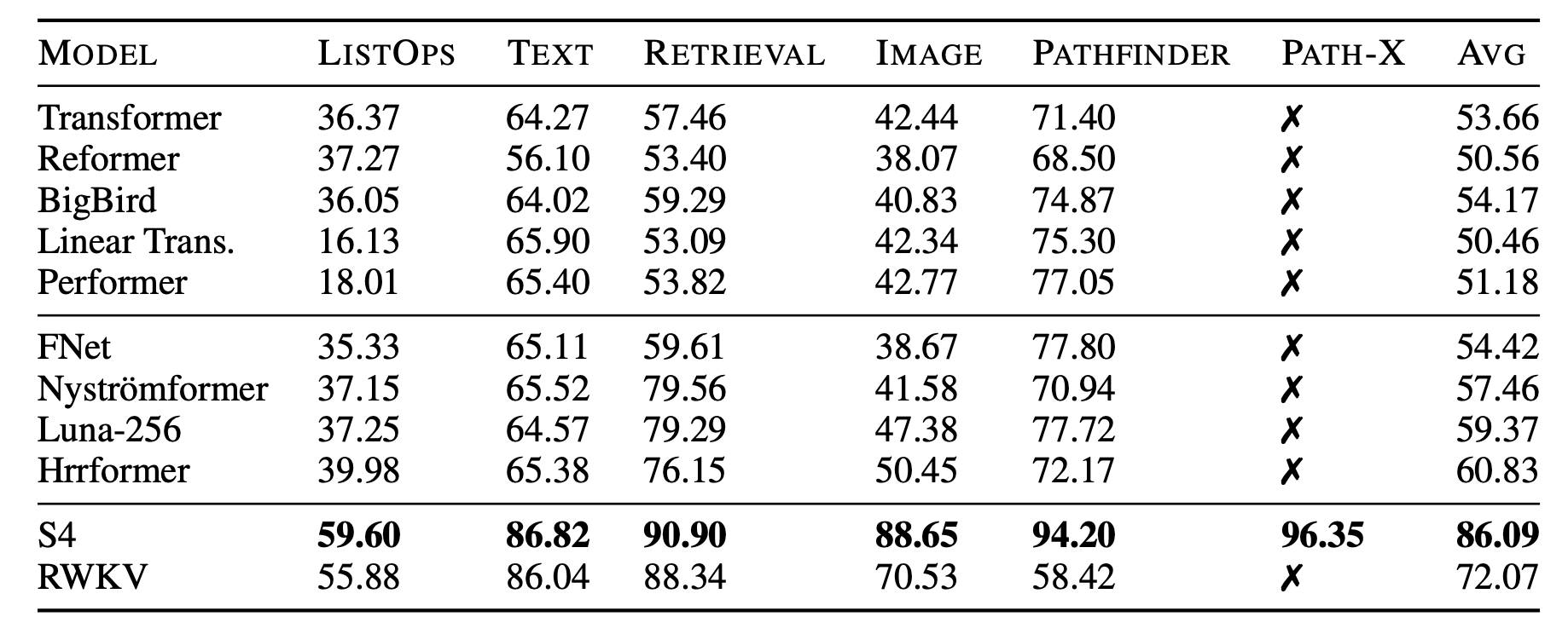
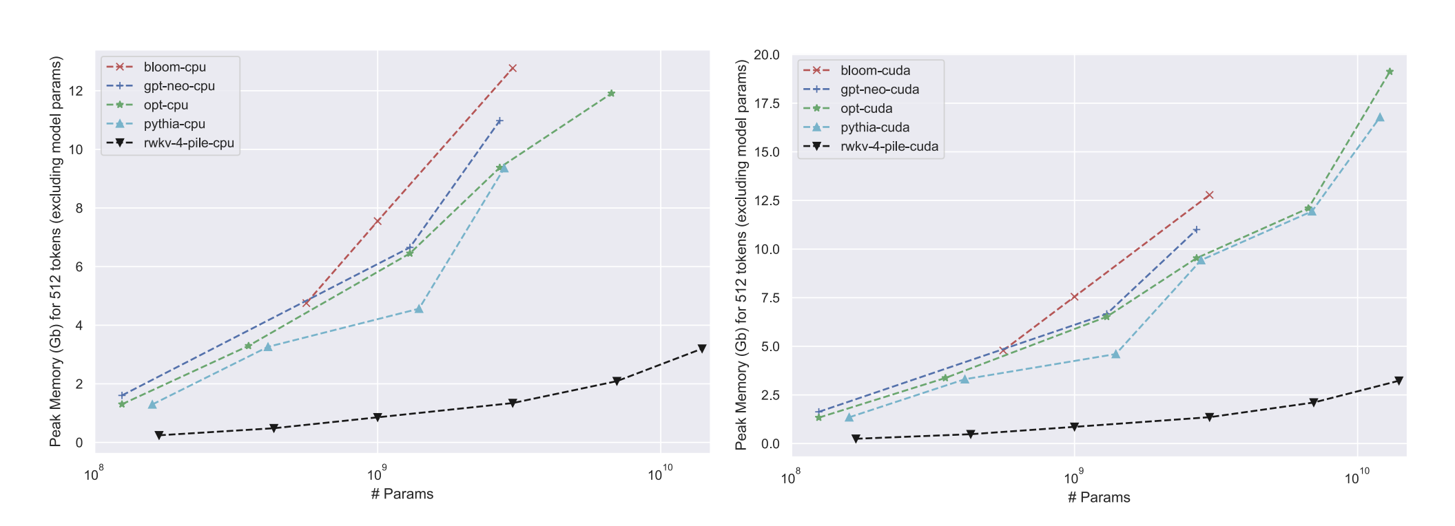
In this post, we discussed the RWKV v4 architecture, which is a linear RNN that allows for efficient computation of attention outputs. We started by introducing the concept of linear attention and its relationship with RNNs. We then discussed the attention-free transformer architecture and its limitations. Finally, we introduced the RWKV v4 architecture, which incorporates several innovations such as the WKV operation, token-shift, and the overall architecture. It turns out that RWKV v4 works very well on long sequences. And it’s memory efficient especially during inference.

What’s next?

• Hardware awareness
• Chunkwise parallelism
• Data dependent decay