In the last three parts of our journey, we solved the parallelism problem with v4’s time-shift, enriched the model’s memory with v5’s matrix-valued states, and made that memory context-aware with v6’s dynamic decay. Each step made the model faster and smarter.
But a fundamental question lurked beneath the surface, a question that haunted all linear-style attention models. The state update in RWKV-4/5/6, at its core, was additive. At each step, we added new information (k*v) and applied a decay w to the entire state.
Think of the model’s memory as a bucket of water. Each new token is a scoop of colored dye. The decay w is like some of the water evaporating, but the colors that are already mixed in stay mixed. Over time, the bucket becomes a muddy, indistinct brown. There was no way to reach in and remove just the red dye that was added 100 steps ago. This “muddying” effect limits how cleanly a model can handle long, complex sequences with distinct pieces of information.
The solution comes from a classic idea in machine learning, revitalized for the modern age: the Delta Rule. This is the story of RWKV-7 “Goose”—the leap from an additive memory to a truly updatable, mutable state, and the profound theoretical power that this unlocks.
From Adding to Updating: The Delta Rule
The traditional state update in linear attention can be seen as:
$$ S_t = S_{t-1} + v_t^T k_t $$Here, the state $\mathbf{S}$ (a matrix in RWKV-5+) simply accumulates the outer products of keys and values.
The Delta Rule, first proposed by Widrow and Hoff in 1960, frames this differently. It sees the state $\mathbf{S}$ as a set of weights for an online learning problem. The goal is to update $\mathbf{S}$ so that when queried with a key $\mathbf{k}$, it produces the corresponding value $\mathbf{v}$. When a new $(\mathbf{k_t}, \mathbf{v_t})$ pair arrives, we update the state to correct the error on this new example. This update rule, for a single step of gradient descent, is:
$$ S_t = S_{t-1}(I - \alpha k_t^T k_t) + \alpha v_t^T k_t $$Let’s break this down:
- $S_{t-1}(I - \alpha k_t^T k_t)$: This is the “erase” step. We take the old state $S_{t-1}$ and subtract a portion $\alpha$ of the information it holds specifically at the address $k_t$.
- $+ \alpha v_t^T k_t$: This is the “write” step. We add the new information $v_t$ at the address $k_t$.
Instead of just adding, the Delta Rule allows the model to partially replace old information with new information at a specific key. It can finally take the red dye out of the bucket. This is the conceptual heart of RWKV-7.
Generalized Delta Rule
RWKV-7 takes this core idea and supercharges it. The full state evolution looks like this:
$$ S_t = S_{t-1} G_t + v_t^T k_t $$Let’s dissect this. The new $(\mathbf{k_t}, \mathbf{v_t})$ pair is added, but the most interesting part is the state transition matrix $\mathbf{G}_t$, which is applied to the old state $\mathbf{S}_{t-1}$.
$\mathbf{G}_t$ has a special structure called Diagonal Plus Low-Rank (DPLR):
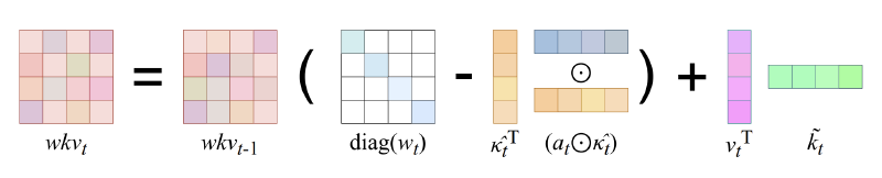
$$ \mathbf{G}_t = \text{diag}(w_t) - \kappa_t^T (\mathbf{a_t} \circ \kappa_t) $$This formula is the engine of RWKV-7. Let’s examine its two components:
$\text{diag}(w_t)$ (The Diagonal Part): This is the per-channel decay we saw in RWKV-6. It’s a diagonal matrix, meaning it applies a separate, data-dependent decay $w_t$ to each feature channel (i.e., each column of the state matrix $\mathbf{S}$). This is our “evaporation” or “forgetting” over time.
$- \kappa_t^T (\mathbf{a_t} \circ \kappa_t)$ (The Low-Rank Part): This is our powerful new “replace” mechanism, derived from the Delta Rule. It’s a rank-1 matrix, which is computationally cheap.
- $\kappa_t$ is the removal key. This vector specifies what information to remove from the state. Crucially, in RWKV-7, this is decoupled from the replacement key $\mathbf{k}_t$. The model can choose to remove information associated with one concept while writing information about another.
- $\mathbf{a_t}$ is the vector-valued in-context learning rate. This is a vector of values between 0 and 1 that controls how much to remove at each channel. It’s also data-dependent. This gives the model fine-grained, per-channel control over the update intensity.
So, at every time step, RWKV-7 performs a sophisticated update:
- It decays the entire memory state $\mathbf{S}_{t-1}$ using the dynamic $\mathbf{w_t}$.
- It surgically removes specific information located at the “address” $\kappa_t$, with an intensity controlled by $\mathbf{a_t}$.
- It then writes new information $\mathbf{v_t}$ at a separate “address” $\mathbf{k_t}$.
This gives the model a flexible, internal scratchpad that it can modify as it processes a sequence.
CUDA Kernel (forward)
| |
A Layman’s Guide to Expressivity: Why This Matters
So, we have a more complex formula. But what does it actually buy us? The answer lies in the esoteric-sounding but deeply important field of computational complexity theory. The question is: What class of problems can a model architecture fundamentally compute?
The Transformer’s Limit: $TC^0$ and the Immutable State
Think of a single layer of a neural network as a computational circuit. For a fixed input length, a Transformer’s attention mechanism can be unrolled into a circuit of logic gates. Researchers have shown that this circuit belongs to a complexity class called $TC^0$.
- What is $TC^0$? It’s the class of problems solvable by circuits with a constant depth (no matter how long the input is) and polynomial size, using threshold gates (e.g., “fire if more than 50% of inputs are active”).
- The Good: This is why Transformers are so parallelizable! A constant-depth circuit can be evaluated extremely quickly.
- The Bad: This is also a fundamental limitation. There are many “simple” problems that are believed to be impossible to solve in $TC^0$, because they require sequential logic.

The core reason for this limitation is that a Transformer’s state—the Key-Value (KV) cache—is immutable. It’s an append-only log. When the model processes token #100, it cannot go back and change what it stored for token #5. It can only choose to attend to it or not.
RWKV-7’s Power: $NC^1$ and the Mutable State
RWKV-7 breaks this barrier. Its state $S_t$ is mutable. The DPLR update rule allows it to fundamentally rewrite its own memory at each step.
Let’s use a simple example to see why this is so powerful: The Swap Problem.
Imagine I give you a list of five items,
[A, B, C, D, E], and then a series of instructions:
- Swap the item in position 1 with the item in position 3. (Now
[C, B, A, D, E])- Swap the item in position 2 with the item in position 5. (Now
[C, E, A, D, B])What is the final order?
A Transformer would find this very difficult. It has to indirectly reason about the changing positions through its attention patterns. An RWKV-7 model, however, can solve this directly. It can initialize its state matrix to be the identity matrix. Each swap instruction causes it to construct a permutation matrix (which is a DPLR matrix!) and multiply its current state by it. The final state matrix is the permutation that describes the final ordering.
This problem is known to be in a higher complexity class called $NC^1$ (problems solvable by logarithmic-depth circuits), which is strongly believed to be more powerful than $TC^0$. By solving this, RWKV-7 proves it is fundamentally more expressive than a Transformer.
The Punchline: Recognizing Any Regular Language
This theoretical power has a stunning consequence, proven in the RWKV-7 paper:
RWKV-7 can recognize any regular language with a constant number of layers.
A regular language is any language that can be described by a Deterministic Finite Automaton (DFA)—a simple state machine. Think about validating an email address, parsing a simple log file, or tracking the state of a game. These are all regular languages.
The ability to simulate any DFA means RWKV-7 has the theoretical machinery to perfectly track finite states and recognize rule-based patterns, a task essential for logical reasoning and structured data understanding. Classical RNNs could theoretically do this, but suffered from vanishing gradients and couldn’t be trained in parallel. Transformers fundamentally cannot. RWKV-7 is the first architecture to achieve this theoretical power while retaining the parallel training and efficient inference of the RWKV family.
This isn’t just a theoretical curiosity. This newfound expressive power, born from the mathematics of the generalized delta rule, is what fuels the state-of-the-art performance we see from RWKV-7 on benchmarks. The theory finally explains the performance, bridging the gap between abstract formulas and real-world results.
Deeper Insight: RWKV-7 as a Fast Weight Programmer
This ability to simulate a state machine is a powerful result, but it’s a symptom of an even deeper principle at play. RWKV-7 isn’t just a state machine; it’s a form of programmable computer. To understand this, we need to introduce the concept of Fast Weight Programming.
In a typical neural network, the “weights” (or parameters) are learned slowly over a massive dataset through gradient descent. We can call these slow weights. The idea of a “fast weight programmer,” pioneered by Jürgen Schmidhuber, is that a network can also have a second set of weights—fast weights—that are rapidly modified within a single forward pass. These fast weights are stored in the network’s hidden states and act as a temporary, context-specific program.
This is exactly what RWKV-7 does. The state matrix $\mathbf{S}_t$ is the set of fast weights. It represents a temporary linear model that is constructed and modified on the fly. The key insight is this: the state update is not an arbitrary rule, but an implementation of online gradient descent on these fast weights.
The Gradient Descent of Fast Weights
Let’s derive this from first principles. Imagine the state matrix $\mathbf{S}_{t-1}$ is our current “program” or internal model. Its job is to map keys to values. When the next token arrives, it gives us a new target mapping: the key $\mathbf{k}_t$ should map to the value $\mathbf{v}_t$.
How well does our current program $\mathbf{S}_{t-1}$ perform on this new task? We can measure the error with a simple loss function, the squared error:
$$ \mathcal{L}(\mathbf{S}_{t-1}) = \frac{1}{2} || \mathbf{S}_{t-1}^T \mathbf{k}_t - \mathbf{v}_t ||_2^2 $$Our goal is to update our program from $\mathbf{S}_{t-1}$ to $\mathbf{S}_t$ by taking a single step of gradient descent to reduce this error. The standard gradient descent update rule is:
$$ \text{New Weights} = \text{Old Weights} - (\text{learning rate}) \times \nabla_{\text{Old Weights}} \mathcal{L} $$In our case, the “weights” are the fast weights in the matrix $\mathbf{S}_{t-1}$.
Let’s find the gradient of our loss function with respect to $\mathbf{S}_{t-1}$:
$$ \nabla_{\mathbf{S}} \mathcal{L} = (\mathbf{S}_{t-1}^T \mathbf{k}_t - \mathbf{v}_t) \mathbf{k}_t^T $$Now, we plug this gradient into our update rule. Let’s use $\alpha$ as our scalar learning rate:
$$ \mathbf{S}_t = \mathbf{S}_{t-1} - \alpha \left( (\mathbf{S}_{t-1}^T \mathbf{k}_t - \mathbf{v}_t) \mathbf{k}_t^T \right)^T $$$$ \mathbf{S}_t = \mathbf{S}_{t-1} - \alpha \mathbf{k}_t (\mathbf{k}_t^T \mathbf{S}_{t-1} - \mathbf{v}_t^T) $$Rearranging the terms, we get:
$$ \mathbf{S}_t = \mathbf{S}_{t-1} - \alpha \mathbf{k}_t \mathbf{k}_t^T \mathbf{S}_{t-1} + \alpha \mathbf{k}_t \mathbf{v}_t^T $$Factoring out $\mathbf{S}_{t-1}$ on the right, we arrive at a familiar formula:
$$ \mathbf{S}_t = (I - \alpha \mathbf{k}_t \mathbf{k}_t^T) \mathbf{S}_{t-1} + \alpha \mathbf{v}_t \mathbf{k}_t^T $$This is precisely the Delta Rule. The “erase” and “write” operations are not just an intuitive idea; they are the direct mathematical consequence of performing one step of gradient descent on the fast weights to learn the new key-value association.
From Delta Rule to RWKV-7’s Full Power
RWKV-7 takes this foundational principle and generalizes it for maximum expressivity:
- Global Forgetting: It introduces the per-channel decay
diag(w_t), combining the gradient descent update with a mechanism to forget information globally over time. - Vector-Valued Learning Rate: The scalar learning rate $\alpha$ is promoted to a data-dependent vector $\mathbf{a}_t$. This allows the model to learn how much to update for each feature channel independently.
- Decoupled Keys: The key used for calculating the error gradient (the “erase” key, $\kappa_t$) is decoupled from the key used for the value to be written ($\mathbf{k}_t$). This adds another layer of flexibility.
Combining these gives us the full RWKV-7 state transition matrix $\mathbf{G}_t = \text{diag}(\mathbf{w}_t) - \kappa_t^T (\mathbf{a}_t \circ \kappa_t)$.
This re-framing is critical. A Transformer learns a static function for processing data. RWKV-7 learns a learning algorithm (the slow weights) that it then executes during the forward pass to rapidly program a temporary, specialized linear model (the fast weights) perfectly adapted to the immediate context. It is a model that learns how to learn, and this meta-learning capability, derived from the mathematics of online gradient descent, is the ultimate source of its power and expressivity.