Linear Attention Basics

In the previous post, we discussed the traditional softmax attention mechanism and its limitations—specifically the $O(n^2)$ computation cost during inference. We also reviewed “classic” RNNs, which boast $O(n)$ inference costs but suffer from a lack of parallelizability during training.

Now, let’s explore a fascinating duality:

1. Attention without softmax $\approx$ RNN
2. RNN with a rank-1 hidden matrix (and no non-linearities inside the recurrence) $\approx$ Attention

This is a pivotal realization. It bridges the gap between parallel training and efficient inference.

Derivation

Attention $\rightarrow$ RNN

Let’s revisit the standard softmax attention mechanism (omitting the scaling factor $d_k$ for simplicity):

If we remove the softmax operation and simply use the raw dot products (a form of “Linear Attention”), the equation becomes:

By defining two cumulative terms, the numerator state $\mathbf{S}_t$ and the denominator state $\mathbf{Z}_t$:

We can rewrite the calculation recursively:

This is, by definition, a linear RNN!

RNN $\rightarrow$ Attention

Conversely, let’s start with a simple RNN formulation:

If we set $\mathbf{W}_h = \mathbf{I}$ (identity matrix), and define the input function as $f_I(\mathbf{x}_t) = \mathbf{k}_t^T \mathbf{v}_t$ (producing a $d \times d$ rank-1 matrix), the hidden state $\mathbf{H}_t$ becomes a matrix rather than a vector.

Unrolling this RNN through time yields:

This is exactly the attention output (a linear combination of value vectors)!

So what?

This result allows us to have the best of both worlds: we can train the model in “Attention Mode” (parallelizable) and switch to “RNN Mode” for inference (constant memory and time).

Furthermore, look at the computational complexity. By dropping softmax and using the associativity of matrix multiplication:

• Standard Attention: computes $(\mathbf{Q}\mathbf{K}^T)\mathbf{V}$, taking $O(n^2d)$ operations.
• Linear Attention: computes $\mathbf{Q}(\mathbf{K}^T\mathbf{V})$, taking $O(nd^2)$ operations.

For long sequence lengths $n$, where $n \gg d$, Linear Attention is significantly faster.

Spoiler: What if we have a causal mask? Standard matrix associativity breaks down with causal masking in a way that makes naive parallelization difficult. RWKV solves this, as we will see in the next post.

Attention Free Transformer (AFT)

Before analyzing RWKV, we must acknowledge the Attention-Free Transformer (AFT), a direct predecessor that offers key insights.

AFT-Simple

The AFT-Simple architecture is defined as:

Here, $\sigma_q$ is a non-linearity (typically sigmoid), and $\odot$ denotes element-wise multiplication. Because the summation terms are independent of $t$, they can be cached, reducing the hidden state to a vector and the cost to $O(n)$.

The RNN form of AFT-Simple is:

AFT-Full

AFT-Full introduces a learnable “pair-wise position bias” $w_{t,j}$:

The term $w_{t,j}$ acts as a learned interaction or gate between position $t$ and position $j$. However, because $w_{t,j}$ depends on both time steps, AFT-Full cannot be unfolded into a simple RNN, and the computation cost reverts to $O(n^2)$.

RWKV v4

Enter RWKV v4. It shares similarities with AFT-Full but introduces crucial modifications to restore $O(n)$ complexity and improve performance:

1. Vector-based Decay: The scalar position bias is replaced by a channel-wise vector $\mathbf{w}$.
2. Relative Decay: Instead of a full $N \times N$ bias matrix, RWKV uses a relative decay $e^{-(t-1-j)w}$ that depends only on the distance between tokens.
3. Bonus Vector: A parameter $\mathbf{u}$ is added to give special attention to the current token, compensating for potential signal degradation in the recurrent state.

The WKV Operation

The core of the architecture is the causal WKV operation:

Unlike AFT, the influence of past tokens decays exponentially as they get further away, controlled by $w$. This acts as a “forgetting” mechanism, similar to the forget gate in an LSTM, but strictly linear and channel-independent.

The RNN Form: Written recursively, the WKV operation becomes:

Numerical Stability: Exponentials like $e^{k_t}$ can grow very large, leading to floating-point overflow. RWKV implements a “log-space” trick, keeping a running maximum $p_t$ to normalize values into a safe range $(0, 1]$:

The official CUDA kernel demonstrates this parallel implementation per channel:

 1
 2
 3
 4
 5
 6
 7
 8
 9
10
11
12
13
14
15
16
17
18
19
20
21
22
23
24

// RWKV v4 WKV operation (forward) - Simplified snippet
template <typename F>
__global__ void kernel_forward(...) {
    // ... setup ...
    F p = 0, q = 0, o = MIN_VALUE;
    
    for (int i = 0; i < T; i++) {
        const int ii = i * C;

        // Calculate Output (applying 'u' bonus)
        F no = max(o, u + k[ii]);
        F A = exp(o - no);
        F B = exp(u + k[ii] - no);
        y[ii] = (A * p + B * v[ii]) / (A * q + B);

        // Update State (applying 'w' decay)
        no = max(w + o, k[ii]);
        A = exp(w + o - no);
        B = exp(k[ii] - no);
        p = A * p + B * v[ii];
        q = A * q + B;
        o = no;
    }
}

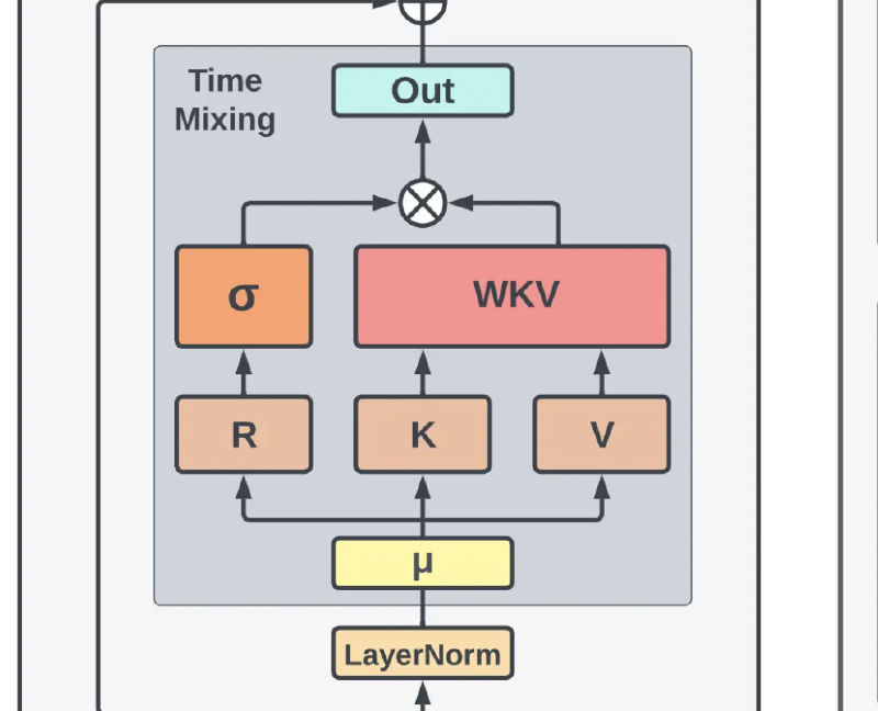
The output is then passed through a gating mechanism: $o_t = W_o \cdot (\sigma(r_t) \odot wkv_t)$, where $R$ (Receptance) acts as the gate for the WKV (Weight-Key-Value) result.

Token-Shift

RWKV v4 introduces “Token-Shift”, a mechanism that mixes the current input with the previous input before the linear layers.

Applied to the inputs for Receptance, Key, and Value:

This acts like a Causal Convolution with kernel size 2. It allows the model to “look back” one step instantly, greatly enhancing its ability to capture local textures and syntax without relying solely on the recurrence.

Note: Mamba later adopted a similar concept (“causal conv1d”) applied to input embeddings before the SSM block.

Overall Architecture

The architecture consists of stacked layers containing:

1. Time Mix: The WKV attention-like operation.
2. Channel Mix: A Feed-Forward Network (FFN) equivalent, also equipped with token-shift.

The Channel Mix block uses a squared-ReLU activation, which has proven effective for this architecture:

Summary

In this post, we traced the evolution from Linear Attention and AFT to RWKV v4. We saw how RWKV acts as a Linear RNN, allowing for $O(1)$ inference cost while maintaining the expressive power of attention through time-decay and token-shifting.

The result is a model that performs exceptionally well on long sequences and is highly memory-efficient.

What’s next?

In the next part, we will discuss optimizations that make RWKV even more powerful:

• Hardware-aware training
• Data-dependent decay

See Eagle and Finch.