Overview
Welcome to this series exploring the RWKV architecture. RWKV is a novel neural network design that merges the efficient inference of Recurrent Neural Networks (RNNs) with the parallelizable training of linear attention mechanisms.
In this series, I will dissect the design and implementation of RWKV. Along the journey, I will also discuss how it relates to other emerging architectures, such as GLA and DeltaNet.
Prerequisite: Traditional Softmax Attention
Before diving into RWKV, we must first review the traditional softmax attention mechanism—the backbone of modern Transformers.
The attention mechanism enables a model to focus on specific parts of an input sequence when making predictions. It computes a weighted sum of input tokens, where the weights are derived from the similarity between a query vector and a set of key vectors.
Given a sequence of $n$ tokens $\mathbf{x} = \begin{bmatrix} \mathbf{x}_1 \ \mathbf{x}_2 \ \vdots \ \mathbf{x}_n \end{bmatrix} \in \mathbb{R}^{n \times d}$, the (non-causal) attention output can be expressed as:
$$ \text{Attn}(t) = \sum_{i=1}^n \alpha(i,t)\mathbf{v}_i=\sum_{i=1}^{n} \frac{\text{sim}(\mathbf{q}_t, \mathbf{k}_i)}{\sum_{j=1}^{n} \text{sim}(\mathbf{q}_t, \mathbf{k}_j)} \mathbf{v}_i=\sum_{i=1}^{n} \frac{\exp(\mathbf{q}_t \mathbf{k}_i^T)}{\sum_{j=1}^{n} \exp(\mathbf{q}_t \mathbf{k}_j^T)} \mathbf{v}_i \in \mathbb{R}^{d} $$Here, $\mathbf{q}_t$, $\mathbf{k}_i$, and $\mathbf{v}_i$ represent the query, key, and value vectors for the $t$-th and $i$-th tokens, respectively. The attention weights $\alpha(i,t)$ are computed using the softmax function, which normalizes the scores to ensure they sum to 1.
Computation Cost
It is easy to see that attention computation has a time complexity of $O(n^2)$. For every token $t$, we must compute attention weights against all $n$ tokens.
This quadratic scaling becomes a significant bottleneck for long sequences. Even during inference with KV caching enabled, the cost of generating a full sequence remains quadratic regarding the sequence length, as the history the model must attend to grows larger with every step.
RNNs
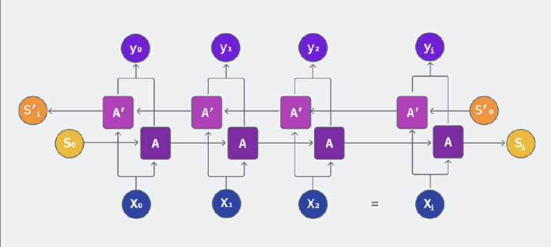
Unlike the attention mechanism, Recurrent Neural Networks (RNNs) process sequences one token at a time, maintaining a hidden state that updates at each time step.
The hidden state is derived from the previous hidden state and the current input token. The formulation is as follows:
$$ \mathbf{h}_t = f(\mathbf{h}_{t-1} \mathbf{W}_{h} + \mathbf{x}_t \mathbf{W}_x+ \mathbf{b}_h) $$$$ \mathbf{y}_t = g(\mathbf{h}_t \mathbf{W}_y + \mathbf{b}_y) $$Where $\mathbf{h}_t$ is the hidden state at time step $t$, and $\mathbf{y}_t$ is the output. The functions $f$ and $g$ are typically non-linear activations. $\mathbf{W}_h$, $\mathbf{W}_x$, and $\mathbf{W}_y$ are the weight matrices for the hidden state, input, and output, respectively, while $\mathbf{b}_h$ and $\mathbf{b}_y$ are the bias vectors.
Computation Cost
Notice that the hidden state $\mathbf{h}t$ depends only on the immediate predecessor $\mathbf{h}{t-1}$ and the current input $\mathbf{x}_t$, rather than the entire history ${\mathbf{h}_0, \mathbf{h}1, \ldots, \mathbf{h}{t-1}}$.
This means that at each time step, the computation cost is $O(1)$ (ignoring the fixed dimensions of the hidden state). Consequently, the total computation cost for processing a sequence of length $n$ is $O(n)$—linear scaling—which is far more efficient than attention mechanisms for long sequences.
Question: Does $O(n)$ mean RNNs are superior?
The short answer is NO. While efficient, traditional RNNs historically failed to replace Transformers. There are two primary reasons why RNNs struggle against softmax attention:
1. Parallelization
Although attention has a higher total computation cost, it can be parallelized across all tokens in the sequence.
Let’s look at the attention equation again:
$$ \text{Attn}(t)=\sum_{i=1}^{n} \frac{\exp(\mathbf{q}_t \mathbf{k}_i^T)}{\sum_{j=1}^{n} \exp(\mathbf{q}_t \mathbf{k}_j^T)} \mathbf{v}_i = \text{softmax}(\mathbf{q}_t \mathbf{K}^T)\mathbf{V} $$In this equation, calculating $\text{Attn}(t)$ does not rely on the output of $\text{Attn}(t-1)$. There are no sequential dependencies on previous time steps during calculation. This allows us to compute the attention output for every token in the sequence simultaneously, offering a massive advantage when training on modern hardware like GPUs or TPUs.
In contrast, RNNs are inherently sequential. To compute the state for token $t$, you must first finish the computation for token $t-1$. This sequential dependency prevents parallel training, leading to significantly longer training times.
2. Long-range Dependencies
RNNs struggle to capture long-range dependencies, particularly in very long sequences.
Because the hidden state $\mathbf{h}_t$ is fixed in size and updated at every step, information from early tokens tends to “vanish” or become diluted as it propagates through the network. Softmax attention, however, has direct access to the entire history (the “global view”), allowing it to recall information from any point in the sequence with equal ease.
Summary
In summary, while RNNs offer lower inference costs ($O(n)$ vs $O(n^2)$), traditional RNNs cannot match the training parallelization or the long-range recall capabilities of Transformers.
In the next post, we will explore how the RWKV architecture solves this dilemma, combining the parallel training of Transformers with the efficient inference of RNNs.
